10. Python を使った数値シミュレーション

前回は統計の基礎について学びました。今回は、その知識を活かしてコンピュータでシミュレーションを行う方法を学んでいきましょう。

10.1 シミュレーションとは？やり方とその意義
10.2 乱数の基礎と random モジュールの使い方
10.3 確率分布とは（一様分布・二項分布・正規分布）
10.4 大数の法則：試行回数を増やすと平均値が一定に近づく
10.5 モンテカルロ法：乱数を使って円周率を求めてみよう
10.6 色々なシミュレーションをしてみよう
10.7 グラフで結果を可視化して考察する
Ex.1 コインを 100 回投げて表と裏の回数を数えるプログラム
Ex.2 サイコロを繰り返し振って、各目の出る確率が 1/6 に近づく様子をグラフ化するプログラム

10.1 シミュレーションとは？やり方とその意義

シミュレーションとは、現実の事象をコンピュータで模擬的に再現する手法です。実験が難しい、コストがかかる、または時間がかかる現象を、コンピュータ上で手軽に何度も試すことができます。

シミュレーションの基本的な考え方

現実の現象をモデル化する
コンピュータ上でそのモデルを実行する
結果を分析して、現実の現象の理解や予測に役立てる

例えば、サイコロを 100 回振った結果を知りたいとき、実際にサイコロを 100 回振るのは大変ですが、コンピュータならすぐに計算できます。

シミュレーションの簡単な例

では、サイコロを 100 回振るシミュレーションを Python で実装してみましょう：

サイコロのシミュレーション

import random

import matplotlib.pyplot as plt
import japanize_matplotlib


results = []

for _ in range(100):
    dice = random.randint(1, 6)  # 1 から 6 までの整数をランダムに生成
    results.append(dice)

# 結果の集計 (count 関数を使って各目の出現回数を数える)
counts = [results.count(i) for i in range(1, 7)]

for number in range(1, 7):
    count = results.count(number)
    percentage = count / len(results) * 100
    print(f"{number}の目: {count}回 ({percentage:.1f}%)")

# 結果をグラフで表示
plt.figure(figsize=(8, 6))
plt.bar(range(1, 7), counts)
plt.title('サイコロを 100 回振った結果')
plt.xlabel('出た目')
plt.ylabel('回数')
plt.xticks(range(1, 7))
plt.grid(axis='y', linestyle='--', alpha=0.7)
plt.show()

サイコロを 100 回振った結果

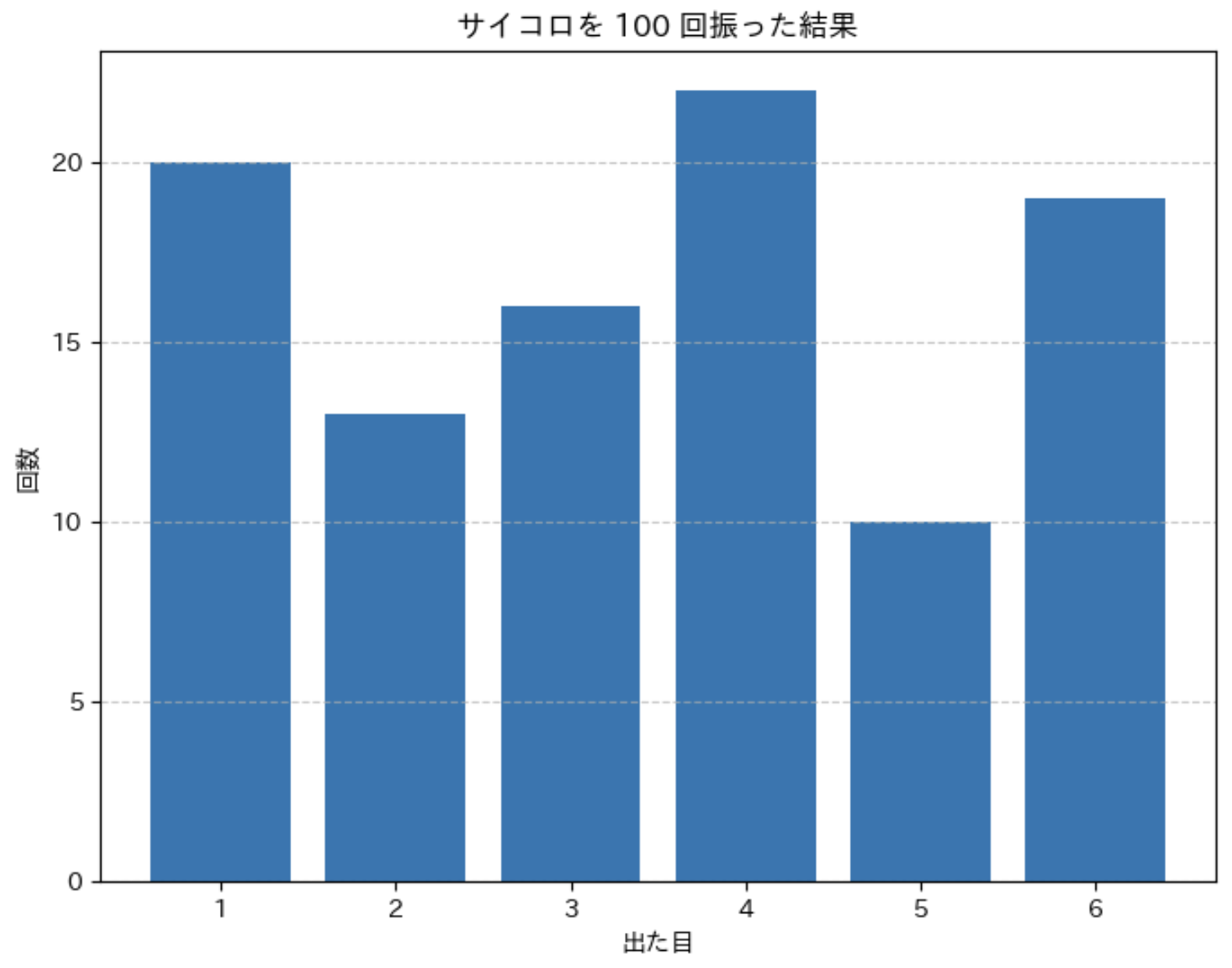
このコードを実行すると、サイコロを 100 回振ったときの各目の出現回数とその割合が表示されます。

理論的には、それぞれの目が約 16.7 %（1 / 6）の確率で出るはずですが、試行回数が 100 回と限られているため、実際の結果にはばらつきが生じます。

10.2 乱数の基礎と random モジュールの使い方

シミュレーションの多くは乱数（ランダムな数値）を使って行われます。

乱数とは？

乱数とは、予測不可能でランダムに生成される数値のことです。

コンピュータが生成する乱数は完全に予測不可能ではないため、正確には「疑似乱数」と呼ばれますが、多くの場合は十分にランダムな性質を持っています。

乱数は、さまざまな場面で使われます。

サイコロやコインのようなランダムな事象のモデル化
ゲームの抽選や、ダメージの計算
確率的なアルゴリズムの実装

Python の random モジュール

Python の標準ライブラリには、乱数を生成するための random モジュールがあります。このモジュールを使うと、様々な種類の乱数を簡単に生成できます。

random モジュールの基本

import random


# 基本的な乱数生成関数
random_float = random.random()  # 0.0 以上 1.0 未満の浮動小数点数
print(f"0 から 1 の乱数: {random_float}")

# 指定範囲の整数乱数
dice = random.randint(1, 6)  # 1 から 6 までの整数
print(f"サイコロの目: {dice}")

# 指定範囲の浮動小数点乱数
temperature = random.uniform(20.0, 30.0)  # 20.0 から 30.0 までの浮動小数点数
print(f"気温: {temperature:.1f}°C")

# 既存のリストからランダムに選択
fruits = ["りんご", "バナナ", "オレンジ", "ぶどう", "メロン"]
chosen_fruit = random.choice(fruits)
print(f"選ばれた果物: {chosen_fruit}")

# リストをシャッフル
cards = ["A", "2", "3", "4", "5", "6", "7", "8", "9", "10", "J", "Q", "K"]
random.shuffle(cards)
print(f"シャッフルされたカード: {cards}")

# 重複なしでランダムに複数選択
lottery_numbers = random.sample(range(1, 46), 6)  # 1 から 45 までの数から重複なしで 6 つ選択
print(f"宝くじの番号: {sorted(lottery_numbers)}")

乱数の種（シード）

乱数生成にはシードと呼ばれる初期値が使われます。同じシードを使えば、同じ乱数列が生成されます。実験の再現性を確保したい（何回実行しても同じ結果にしたい）場合に役立ちます。

乱数のシード設定

import random


# シードを固定
random.seed(42)

# 乱数を生成
for _ in range(5):
    print(random.random())

print("\n同じシードで再度生成:")
# 同じシードを設定すると同じ乱数列が生成される
random.seed(42)

for _ in range(5):
    print(random.random())

10.3 確率分布とは（一様分布・二項分布・正規分布）

確率分布とは、ランダムな事象や変数がどのような値をどのくらいの確率で取るかを表したものです。主な確率分布には以下のようなものがあります。

一様分布（Uniform Distribution）
- 指定された範囲内のすべての値が等しい確率で出現する分布
- サイコロの目やルーレットの数字など
二項分布（Binomial Distribution）
- 成功 / 失敗の 2 種類の結果があるような試行を繰り返したときの分布
- コイン投げなど
正規分布（Normal Distribution）
- つりがね型の分布で、多くの自然現象に当てはまる
- 身長や体重など

一様分布

一様分布は、指定された範囲内のすべての値が等しい確率で出現する分布です。サイコロの目やルーレットの数字などが一様分布の例です。

一様分布のシミュレーション

import random

import numpy as np
import matplotlib.pyplot as plt
import japanize_matplotlib


# 一様分布からの乱数生成
uniform_values = [random.uniform(0, 1) for _ in range(1000)]

# ヒストグラムの描画
plt.figure(figsize=(10, 6))

# ヒストグラムを描画（正規化して確率密度関数として表示）
counts, bins, patches = plt.hist(
    uniform_values,
    bins=20,
    color='skyblue',
    edgecolor='black',
    alpha=0.7,
    density=True,
    label='シミュレーション結果'
)

# 理論値の計算と描画
x = np.linspace(0, 1, 100)
y = np.ones_like(x)  # 一様分布の確率密度関数は区間内で常に 1
plt.plot(x, y, 'r-', linewidth=2, label='理論値')

plt.title('一様分布 (0 から 1 の範囲)', fontsize=14)
plt.xlabel('値', fontsize=12)
plt.ylabel('確率密度', fontsize=12)
plt.grid(True, alpha=0.3)
plt.legend()
plt.show()

# 平均と標準偏差
mean = np.mean(uniform_values)
std_dev = np.std(uniform_values)
print(f"平均: {mean:.4f}")
print(f"標準偏差: {std_dev:.4f}")
print(f"理論上の平均: 0.5")
print(f"理論上の標準偏差: {1/np.sqrt(12):.4f}")

一様分布のヒストグラム

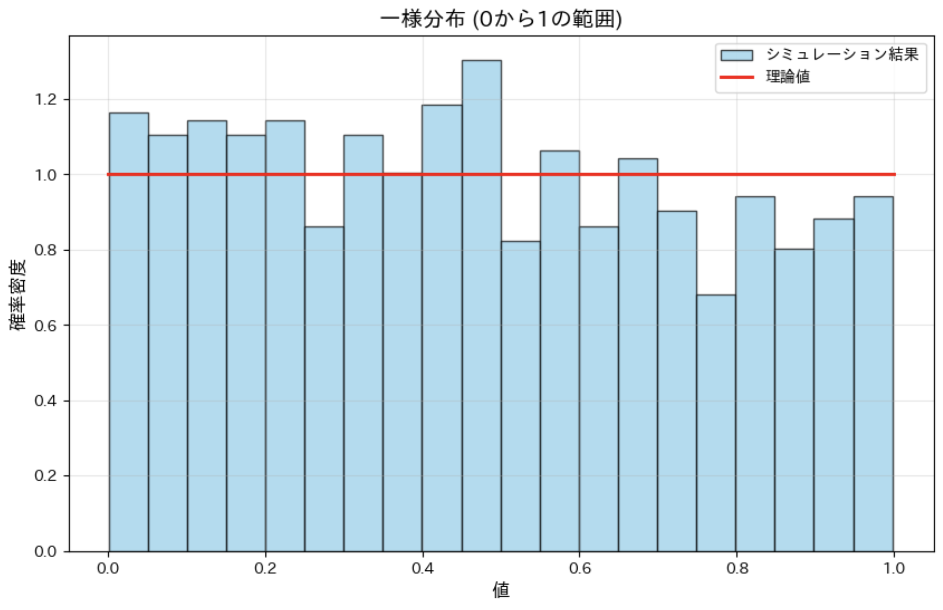
一様分布では、すべての値が等しい確率で出現するため、ヒストグラムはほぼ平らな形になります。0 から 1 の一様分布の理論上の

平均は 0.5
標準偏差は約 0.2887（ $\frac{1}{\sqrt{12}}$ ）

です。

二項分布

二項分布は、成功確率が一定の試行を複数回繰り返したときの成功回数の分布です。コイン投げや合否判定など、成功（表）か失敗（裏）の2種類の結果しかない試行を繰り返す場合に現れます。

二項分布のシミュレーション

import random

import numpy as np
import matplotlib.pyplot as plt
import japanize_matplotlib
from scipy.stats import binom


# コイン投げのシミュレーション （10 回投げて表が出る回数）
def coin_flip_experiment():
    flips = [random.random() < 0.5 for _ in range(10)]  # Trueが表、Falseが裏
    return sum(flips)  # 表の回数を返す

# 1000 回の実験を行う
results = [coin_flip_experiment() for _ in range(1000)]

# ヒストグラムの描画
plt.figure(figsize=(10, 6))
values, counts, _ = plt.hist(results, bins=np.arange(-0.5, 11, 1), color='lightblue', edgecolor='black')

# 理論値の計算と描画
n, p = 10, 0.5  # 試行回数と成功確率
x = np.arange(0, 11)
pmf = binom.pmf(x, n, p)  # 確率質量関数
plt.plot(x, 1000 * pmf, 'ro-', ms=8, label='理論値')

plt.title('二項分布: 10 回のコイン投げで表が出る回数', fontsize=14)
plt.xlabel('表の回数', fontsize=12)
plt.ylabel('頻度', fontsize=12)
plt.xticks(range(11))
plt.legend()
plt.grid(True, alpha=0.3)
plt.show()

# 平均と標準偏差
mean = np.mean(results)
std_dev = np.std(results)
print(f"平均: {mean:.4f}")
print(f"標準偏差: {std_dev:.4f}")
print(f"理論上の平均: {n * p}")
print(f"理論上の標準偏差: {np.sqrt(n * p * (1 - p)):.4f}")

二項分布のヒストグラム

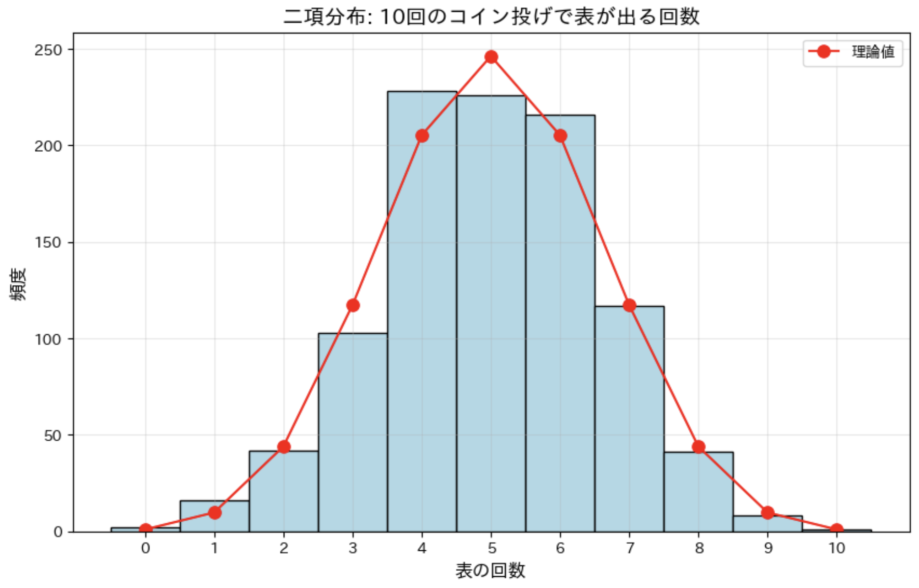
二項分布は、n 回の試行のうち成功する回数の分布です。コイン投げの場合、表が出る確率は 0.5 なので、10 回投げたときの表の回数の

理論上の平均は 5 回
標準偏差は約 1.58（ $\sqrt{10 \times 0.5 \times 0.5}$ ）

です。

正規分布

正規分布（ガウス分布とも呼ばれる）は、釣鐘型の対称な分布で、自然界の多くの現象（身長、体重、テストの点数など）がこの分布に従います。

正規分布のシミュレーション

import numpy as np
import matplotlib.pyplot as plt
import japanize_matplotlib
from scipy.stats import norm


# 正規分布からの乱数生成 （平均 170 cm, 標準偏差 5 cm の身長データ）
heights = np.random.normal(170, 5, 1000)

# ヒストグラムの描画
plt.figure(figsize=(10, 6))
plt.hist(heights, bins=30, color='lightblue', edgecolor='black', density=True)

# 理論的な正規分布曲線の描画
x = np.linspace(150, 190, 1000)
plt.plot(x, norm.pdf(x, 170, 5), 'r-', linewidth=2, label='理論曲線')

plt.title('正規分布: 平均 170cm, 標準偏差 5cm の身長データ', fontsize=14)
plt.xlabel('身長 (cm)', fontsize=12)
plt.ylabel('確率密度', fontsize=12)
plt.legend()
plt.grid(True, alpha=0.3)
plt.show()

# 平均と標準偏差
mean = np.mean(heights)
std_dev = np.std(heights)
print(f"平均: {mean:.4f}cm")
print(f"標準偏差: {std_dev:.4f}cm")

正規分布のヒストグラム

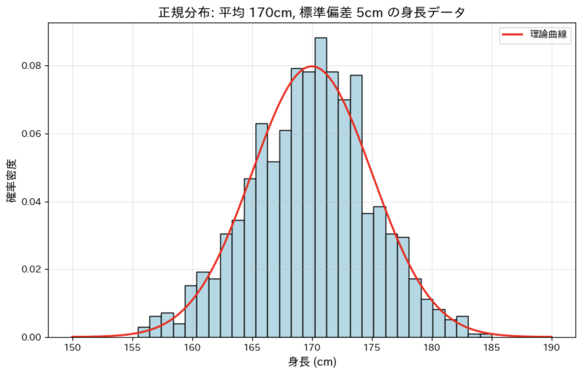
正規分布は平均値を中心に左右対称なつりがね型の分布です。

データの約 68% が平均 ±1 標準偏差の範囲に、約 95% が平均 ±2 標準偏差の範囲に、約 99.7% が平均 ±3 標準偏差の範囲に入ります。

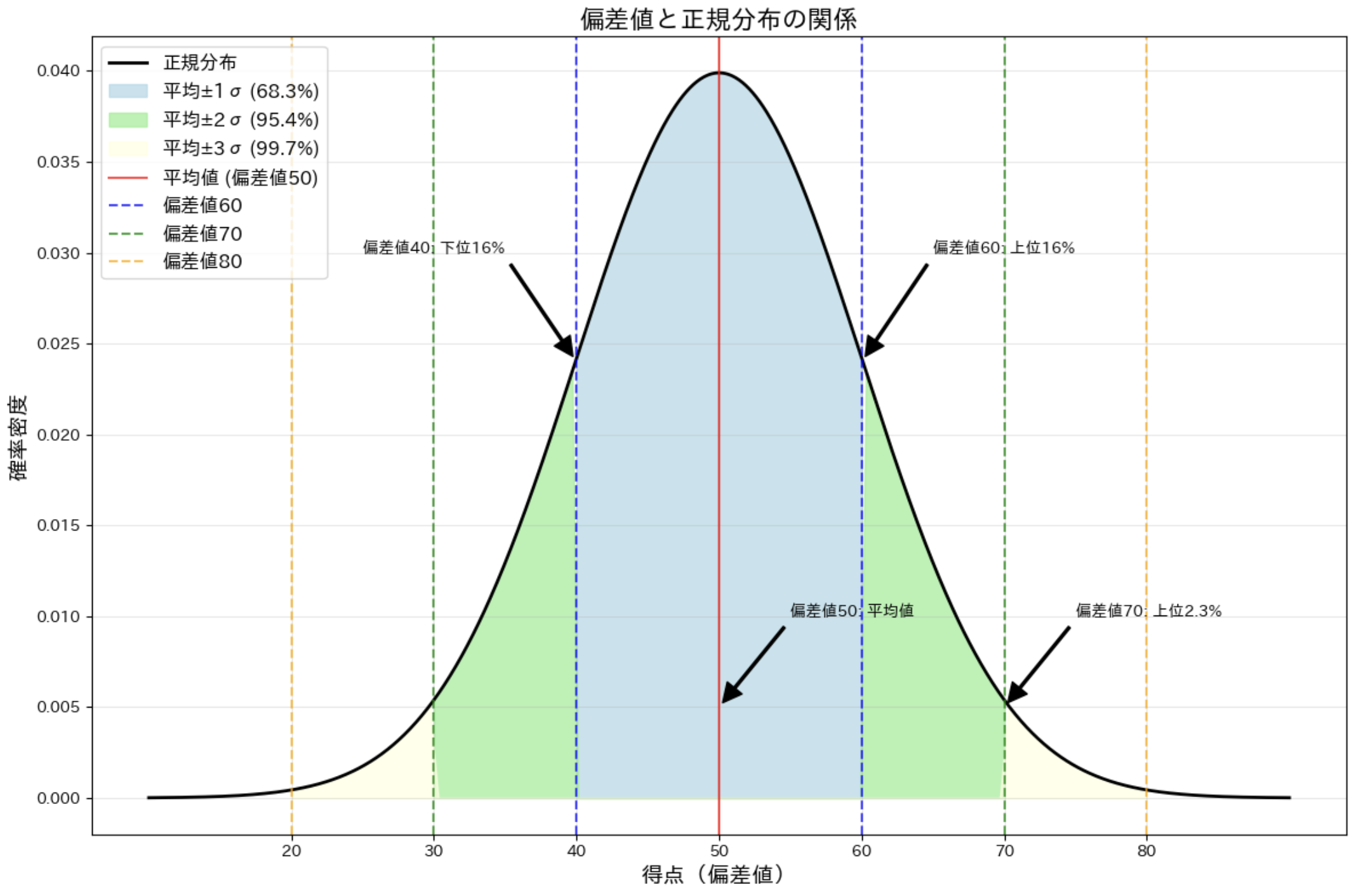
偏差値と正規分布の関係

偏差値は、正規分布に基づいて得点を評価するための指標です。偏差値は、平均値を 50 とし、標準偏差を 10 として計算されます。

偏差値と正規分布の関係

import numpy as np
import matplotlib.pyplot as plt
import japanize_matplotlib
from scipy.stats import norm


# グラフの設定
plt.figure(figsize=(12, 8))

# 正規分布のパラメータ
mu = 50  # 平均
sigma = 10  # 標準偏差

# x 軸の範囲
x = np.linspace(mu - 4 * sigma, mu + 4 * sigma, 1000)

# 正規分布の確率密度関数
pdf = norm.pdf(x, mu, sigma)

# 正規分布曲線をプロット
plt.plot(x, pdf, 'k-', linewidth=2, label='正規分布')

# 平均 ±1 標準偏差 （約 68%） の範囲を塗りつぶす
x_fill_1sigma = np.linspace(mu - sigma, mu + sigma, 100)
plt.fill_between(
    x_fill_1sigma,
    norm.pdf(x_fill_1sigma, mu, sigma),
    color='lightblue',
    alpha=0.7,
    label='平均 ± 1σ (68.3%)'
)

# 平均 ±2 標準偏差 （約 95%） の範囲を塗りつぶす
x_fill_2sigma = np.linspace(mu - 2 * sigma, mu + 2 * sigma, 100)
x_fill_1sigma_mask = (x_fill_2sigma >= mu - sigma) & (x_fill_2sigma <= mu + sigma)
x_fill_2sigma_only = np.copy(x_fill_2sigma)
y_values = norm.pdf(x_fill_2sigma_only, mu, sigma)
y_values[x_fill_1sigma_mask] = 0
plt.fill_between(
    x_fill_2sigma_only,
    y_values,
    color='lightgreen',
    alpha=0.7,
    label='平均 ± 2σ (95.4%)'
)

# 平均 ±3 標準偏差 （約 99.7%） の範囲を塗りつぶす
x_fill_3sigma = np.linspace(mu - 3 * sigma, mu + 3 * sigma, 100)
x_fill_2sigma_mask = (x_fill_3sigma >= mu - 2 * sigma) & (x_fill_3sigma <= mu + 2 * sigma)
x_fill_3sigma_only = np.copy(x_fill_3sigma)
y_values = norm.pdf(x_fill_3sigma_only, mu, sigma)
y_values[x_fill_2sigma_mask] = 0
plt.fill_between(
    x_fill_3sigma_only,
    y_values,
    color='lightyellow',
    alpha=0.7,
    label='平均 ± 3σ (99.7%)'
)

# 偏差値の目盛りを追加
plt.axvline(x=mu, color='red', linestyle='-', alpha=0.7, label='平均値 (偏差値50)')
plt.axvline(x=mu + sigma, color='blue', linestyle='--', alpha=0.7, label='偏差値60')
plt.axvline(x=mu - sigma, color='blue', linestyle='--', alpha=0.7)
plt.axvline(x=mu + 2 * sigma, color='green', linestyle='--', alpha=0.7, label='偏差値70')
plt.axvline(x=mu - 2 * sigma, color='green', linestyle='--', alpha=0.7)
plt.axvline(x=mu + 3 * sigma, color='orange', linestyle='--', alpha=0.7, label='偏差値80')
plt.axvline(x=mu - 3 * sigma, color='orange', linestyle='--', alpha=0.7)

# 軸ラベルとタイトル
plt.title('偏差値と正規分布の関係', fontsize=16)
plt.xlabel('得点（偏差値）', fontsize=14)
plt.ylabel('確率密度', fontsize=14)
plt.xticks(
    [mu - 3 * sigma, mu - 2 * sigma, mu - sigma, mu, mu + sigma, mu + 2 * sigma, mu + 3 * sigma],
    ['20', '30', '40', '50', '60', '70', '80']
)
plt.grid(True, alpha=0.3)
plt.legend(loc='upper left', fontsize=12)

# テキスト注釈を追加
plt.annotate(
    '偏差値 50: 平均値',
    xy=(mu, 0.005),
    xytext=(mu + 5, 0.01),
    arrowprops=dict(facecolor='black', shrink=0.05, width=1.5)
)
plt.annotate(
    '偏差値 60: 上位 16%',
    xy=(mu + sigma, 0.024),
    xytext=(mu + sigma + 5, 0.03),
    arrowprops=dict(facecolor='black', shrink=0.05, width=1.5)
)
plt.annotate(
    '偏差値 70: 上位 2.3%',
    xy=(mu + 2 * sigma, 0.005),
    xytext=(mu + 2 * sigma + 5, 0.01),
    arrowprops=dict(facecolor='black', shrink=0.05, width=1.5)
)
plt.annotate(
    '偏差値 40: 下位 16%',
    xy=(mu-sigma, 0.024),
    xytext=(mu-sigma-15, 0.03),
    arrowprops=dict(facecolor='black', shrink=0.05, width=1.5)
)

plt.tight_layout()
plt.show()

偏差値と正規分布の関係

10.4 大数の法則：試行回数を増やすと平均値が一定に近づく

大数の法則（Law of Large Numbers）とは、試行回数を増やしていくと、結果の平均値が理論上の期待値（確率的な平均値）に近づいていくという法則です。簡単に言えば、「たくさん試せば試すほど、平均値は理論値に近づく」ということです。

例えば：

コイン投げを数回だけすると表の割合は 0.5（50%）から大きくずれることがありますが、何千回も投げると、表の割合は 0.5 に近づいていきます
サイコロを数回振ると平均値は 3.5 から離れることがありますが、何千回も振ると、平均値は3.5に近づいていきます

この法則は、確率論の基本原理の一つであり、統計学やシミュレーションの基礎となっています。

コイン投げでの大数の法則

まず、コイン投げのシミュレーションで大数の法則を確認してみましょう。

コイン投げの大数の法則

import random

import numpy as np
import matplotlib.pyplot as plt
import japanize_matplotlib


def coin_flip_simulation(trials):
    """コイン投げをシミュレーションし、各試行後の表の割合を記録"""
    heads = 0  # 表の回数
    heads_ratio = []  # 表の割合の履歴

    for i in range(1, trials + 1):
        # コインを投げる （0.5 の確率で表）
        if random.random() < 0.5:
            heads += 1

        # i 回目の試行後の表の割合を記録
        heads_ratio.append(heads / i)

    return heads_ratio


# 異なる試行回数でシミュレーション
trials_100 = coin_flip_simulation(100)
trials_1000 = coin_flip_simulation(1000)
trials_10000 = coin_flip_simulation(10000)

# グラフの描画
plt.figure(figsize=(12, 6))

# 各シミュレーション結果をプロット
plt.plot(range(1, 101), trials_100, label='100 回試行', alpha=0.7)
plt.plot(range(1, 1001), trials_1000, label='1,000 回試行', alpha=0.7)
plt.plot(range(1, 10001), trials_10000, label='10,000 回試行', alpha=0.7)

# 理論値（0.5）の水平線
plt.axhline(y=0.5, color='r', linestyle='--', label='理論値(0.5)')

# グラフの装飾
plt.xscale('log')  # x軸を対数スケールに
plt.xlabel('試行回数', fontsize=12)
plt.ylabel('表の出る割合', fontsize=12)
plt.title('コイン投げシミュレーション：大数の法則', fontsize=14)
plt.legend()
plt.grid(True, alpha=0.3)

# 範囲を制限して見やすく
plt.ylim(0.3, 0.7)

plt.show()

# 最終的な表の割合
print(f"100 回試行後の表の割合: {trials_100[-1]:.4f}")
print(f"1,000 回試行後の表の割合: {trials_1000[-1]:.4f}")
print(f"10,000 回試行後の表の割合: {trials_10000[-1]:.4f}")

コイン投げの大数の法則

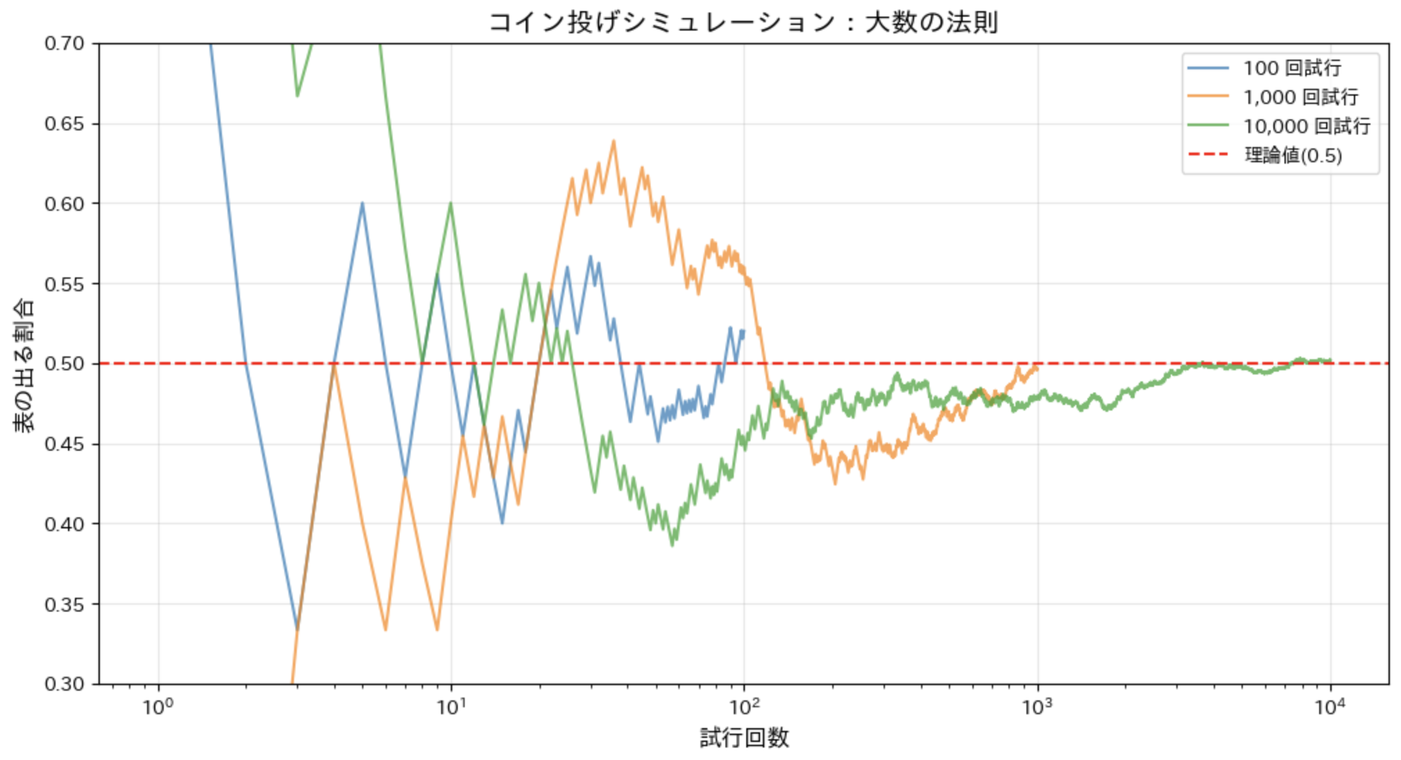
このシミュレーションでは、コイン投げを 100 回, 1,000 回, 10,000 回行い、各試行後の表の割合を記録しています。グラフを見ると、試行回数が増えるにつれて表の割合が理論値である 0.5 に近づいていることがわかります。

10.5 モンテカルロ法：乱数を使って円周率を求めてみよう

先ほどの大数の法則を応用した手法の一つに「モンテカルロ法」があります。

モンテカルロ法とは？

モンテカルロ法（Monte Carlo Method）は、乱数を使った統計的シミュレーションによって複雑な問題を解く手法です。この手法は以下のような特徴を持っています。

乱数を多数生成して確率的なシミュレーションを行う
大数の法則に基づいて、シミュレーション結果から求めたい値を近似する
解析的に解くのが難しい複雑な問題に対して有効

円周率の計算：モンテカルロ法の基本例

モンテカルロ法の最も有名な例の一つが、円周率（ $\pi$ ）の計算です。この方法は、正方形の中に描かれた円に乱数で生成した点がどれだけ入るかを数えることで、 $\pi$ を近似します。

アイデアは単純です：

正方形の中に円を描く
正方形内にランダムな点を多数打つ
円の内側に入った点の割合から円周率を計算する

数学的には、半径 1 の四分割した円の面積は $\frac{\pi}{4}$ であり、一辺が 1 の正方形の面積は 1 です。

したがって、ランダムな点が四分割した円の内側に入る確率は、

\frac{\text{円の面積}}{\text{正方形の面積}} = \frac{\pi}{4}

となります。

よって、

\pi = 4 \times \frac{\text{円の内側に入った点の数}}{\text{正方形の中に打たれた点の数}}

という式が成り立ちます。

モンテカルロ法による円周率の計算

import random

import numpy as np
import matplotlib.pyplot as plt
import japanize_matplotlib


def estimate_pi(num_points):
    """モンテカルロ法で円周率を推定する"""
    inside_circle = 0  # 円の内側に入った点の数

    # 点のデータを保存するためのリスト
    x_inside, y_inside = [], []  # 円の内側の点
    x_outside, y_outside = [], []  # 円の外側の点

    # num_points 個のランダムな点を生成
    for _ in range(num_points):
        x = random.random()  # 0 から 1 の乱数
        y = random.random()  # 0 から 1 の乱数

        # 点が円の内側かどうか判定 （x ^ 2 + y ^ 2 <= 1 なら内側）
        if x * x + y * y <= 1:
            inside_circle += 1
            x_inside.append(x)
            y_inside.append(y)
        else:
            x_outside.append(x)
            y_outside.append(y)

    # 円周率の推定値を計算
    pi_estimate = 4 * inside_circle / num_points

    return pi_estimate, x_inside, y_inside, x_outside, y_outside

# 一度に計算する点の数
num_points = 10000

# 円周率を推定
pi_estimate, x_in, y_in, x_out, y_out = estimate_pi(num_points)

# 結果を表示
print(f"点の数: {num_points}")
print(f"円の内側に入った点の数: {len(x_in)}")
print(f"推定された円周率: {pi_estimate}")
print(f"実際の円周率との誤差: {abs(pi_estimate - np.pi)}")

# 点をプロット
plt.figure(figsize=(8, 8))
plt.scatter(x_in, y_in, color='blue', s=1, alpha=0.6, label='円の内側')
plt.scatter(x_out, y_out, color='red', s=1, alpha=0.6, label='円の外側')

# 四分割した円を描画
theta = np.linspace(0, np.pi / 2, 100)
plt.plot(np.cos(theta), np.sin(theta), 'g-', linewidth=2)

# グラフの設定
plt.axis('equal')
plt.xlim(0, 1)
plt.ylim(0, 1)
plt.title(f'モンテカルロ法による円周率の計算\n推定値: {pi_estimate:.6f}（点の数: {num_points}）', fontsize=14)
plt.legend()
plt.grid(True, alpha=0.3)
plt.show()

モンテカルロ法による円周率の計算

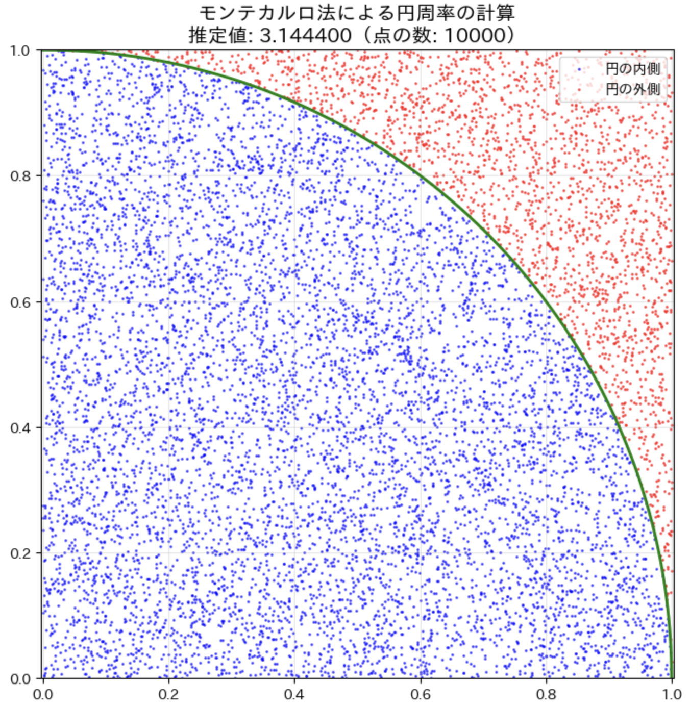
このコードでは、10,000 個のランダムな点を生成し、円の内側に入った点の数から円周率を推定しています。

結果は実際の円周率（ $\pi \approx 3.1415...$ ）に近い値になるはずです。これも大数の法則に従って、点の数が増えるほど精度が上がります。

10.6 色々なシミュレーションをしてみよう

ここでは、実際の問題に近い形でシミュレーションについて学びましょう。

在庫管理シミュレーション

商品の在庫管理に関するシミュレーションを考えてみましょう。

ある小売店では、人気商品Aの在庫管理方法を検討しています。以下の条件でシミュレーションを行うことにしました。

初期在庫数は 10 個
毎日の需要は 0 〜 5 個の範囲でランダム
在庫が 5 個以下になったら 10 個を追加発注する
発注してから商品が到着するまでに 3 日かかる
30 日間のシミュレーションを行う

発注のしきい値と発注数を変えながらシミュレーションを実行し、品切れ日数が 0 になるパラメータを探してみましょう。

このシミュレーションを Python で実装してみましょう。

在庫管理シミュレーション

import random


def simulate_inventory(
    days: int = 30,
    initial_stock: int = 10,
    reorder_threshold: int = 5,
    reorder_amount: int = 10,
    lead_time: int = 3,
) -> tuple[list[int], list[int], int]:
    """在庫管理シミュレーション.

    Args:
        days (int): シミュレーション日数
        initial_stock (int): 初期在庫数
        reorder_threshold (int): 発注する在庫数のしきい値
        reorder_amount (int): 発注数
        lead_time (int): 発注から到着までの日数

    Returns:
        tuple[list[int], list[int], int]: (在庫履歴, 注文中リスト履歴, 品切れ日数)
    """
    stock = initial_stock
    pending_orders = []  # (到着予定日, 発注数) のリスト
    stock_history = [stock]
    pending_history = [len(pending_orders)]
    stockout_days = 0

    print(f"初期状態: 在庫数 = {stock}, 発注中 = {pending_orders}")

    for day in range(1, days + 1):
        print(f"\n--- 日付: {day} ---")

        # 注文が到着する場合
        new_pending = []
        arrived_orders = []

        for arrival_day, amount in pending_orders:
            if day >= arrival_day:
                stock += amount
                arrived_orders.append((arrival_day, amount))
            else:
                new_pending.append((arrival_day, amount))

        if arrived_orders:
            for arrival_day, amount in arrived_orders:
                print(f"注文到着: {amount}個 (発注日: {arrival_day - lead_time})")

        pending_orders = new_pending

        # 今日の需要
        demand = random.randint(0, 5)
        print(f"本日の需要: {demand}個")

        # 在庫から出荷
        if stock >= demand:
            stock -= demand
            print(f"出荷完了: 残り在庫 = {stock}個")
        else:
            # 在庫不足の場合
            print(f"在庫不足! 要求: {demand}個, 在庫: {stock}個")
            stockout_days += 1
            stock = 0

        # 発注判断
        if stock <= reorder_threshold and not pending_orders:
            pending_orders.append((day + lead_time, reorder_amount))
            print(f"発注実行: {reorder_amount}個 (到着予定日: {day + lead_time})")

        # 履歴を記録
        stock_history.append(stock)
        pending_history.append(len(pending_orders))

        # 現在の状況サマリー
        print(f"日終了時点: 在庫数 = {stock}個, 発注中 = {[(d, a) for d, a in pending_orders]}")

    print("\n--- シミュレーション終了 ---")

    return stock_history, pending_history, stockout_days


# シミュレーションを実行
stock_history, pending_history, stockout_days = simulate_inventory()
print(f"\n30 日間の品切れ日数: {stockout_days}日")
print(f"最終在庫: {stock_history[-1]}個")
print(f"在庫推移: {stock_history}")
print(f"発注中数推移: {pending_history}")

10.7 グラフで結果を可視化して考察する

シミュレーション結果をただ数値で見るだけでは、傾向や特徴を把握するのが難しい場合があります。データを可視化することで、より直感的に結果を理解し、考察することができます。

在庫管理シミュレーションの可視化

在庫管理シミュレーションの結果を可視化してみましょう。

在庫管理シミュレーションの可視化

import numpy as np
import matplotlib.pyplot as plt
import japanize_matplotlib


def visualize_inventory_simulation(
    reorder_thresholds: list[int] = [5, 10, 15],
    reorder_amounts: list[int] = [5, 10, 15],
) -> None:
    """在庫管理シミュレーションの可視化.

    Args:
        reorder_thresholds (list[int]): 試す発注しきい値のリスト
        reorder_amounts (list[int]): 試す発注数のリスト
    """
    fig, axes = plt.subplots(len(reorder_thresholds), len(reorder_amounts), figsize=(15, 10))

    stockout_results = np.zeros((len(reorder_thresholds), len(reorder_amounts)))

    for i, threshold in enumerate(reorder_thresholds):
        for j, amount in enumerate(reorder_amounts):
            # 先ほど定義した関数を使用
            stock_history, pending_history, stockout_days = simulate_inventory(
                days=30,
                initial_stock=10,
                reorder_threshold=threshold,
                reorder_amount=amount,
                lead_time=3
            )

            ax = axes[i, j]
            days = range(31)  # 0 日目を含む

            ax.plot(days, stock_history, 'b-', label='在庫数')
            ax.set_title(f'しきい値={threshold}, 発注数={amount}\n品切れ={stockout_days}日')
            ax.set_ylim(0, max(max(stock_history) + 2, 20))
            ax.grid(True)

            if i == len(reorder_thresholds) - 1:
                ax.set_xlabel('日数')
            if j == 0:
                ax.set_ylabel('在庫数')

            stockout_results[i, j] = stockout_days

    plt.tight_layout()
    plt.show()


visualize_inventory_simulation()

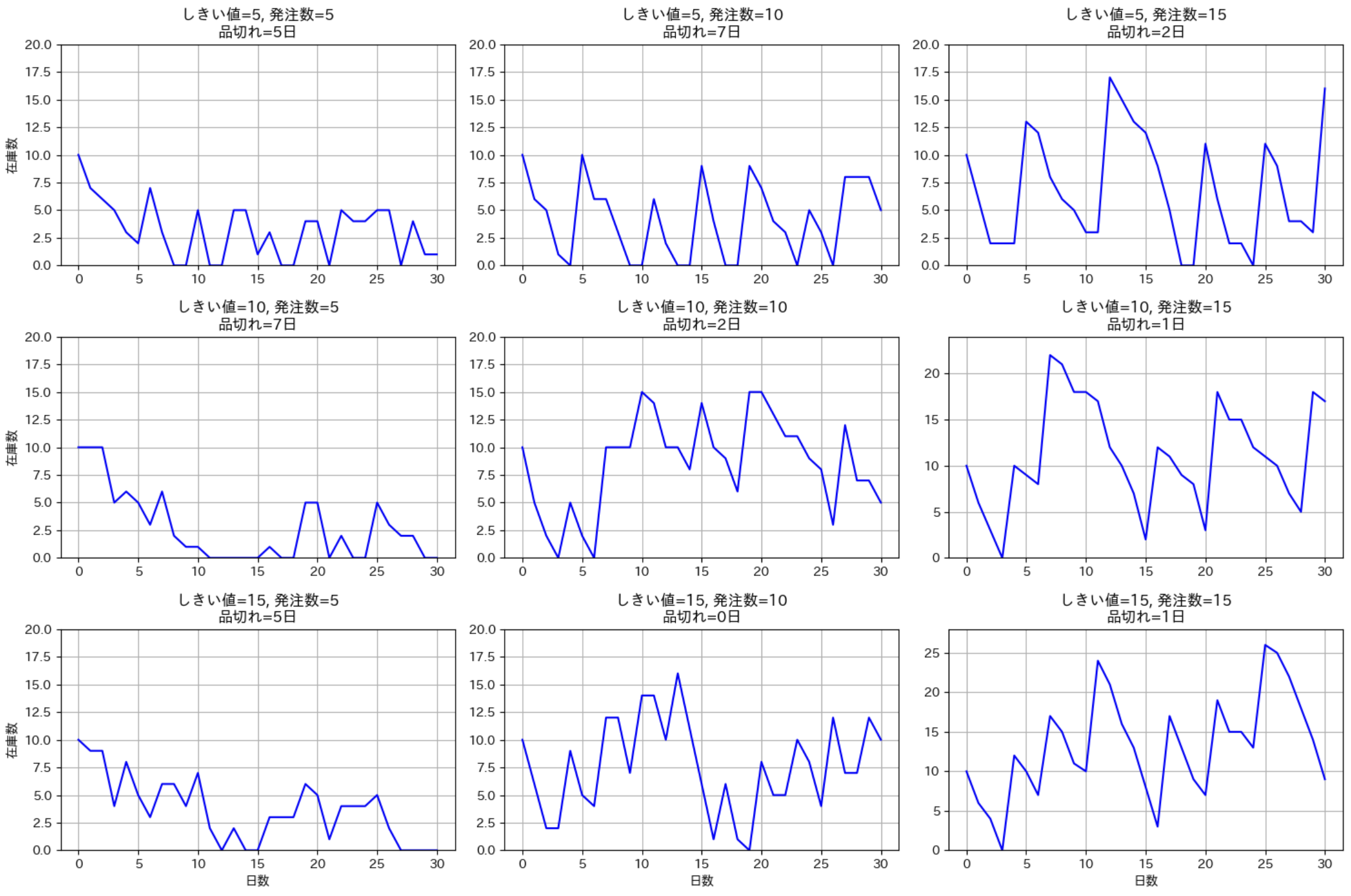
この可視化では、発注しきい値（何個以下になったら発注するか）と発注数の様々な組み合わせに対する在庫の推移と品切れ日数を確認できます。

Ex.1 コインを 100 回投げて表と裏の回数を数えるプログラム

コイン投げシミュレーション

import random
from collections import Counter

import matplotlib.pyplot as plt
import japanize_matplotlib


def coin_flip_experiment(flips: int = 100) -> Counter:
    # コインを指定回数投げる
    results = []
    for _ in range(flips):
        result = '裏' if random.random() < 0.5 else '表'
        results.append(result)

    # 結果を集計
    count = Counter(results)

    # 結果を表示
    print(f"\n{flips}回コインを投げた結果:")
    for face, num in count.items():
        percentage = (num / flips) * 100
        print(f"{face}: {num}回 ({percentage:.1f}%)")

    # グラフの作成
    plt.figure(figsize=(8, 6))
    plt.bar(count.keys(), count.values())
    plt.title(f'コイン投げの結果 ({flips}回)')
    plt.ylabel('回数')
    plt.show()

    return count


result = coin_flip_experiment(100)

チャレンジ：

複数回実験を行い、結果の平均を取ってみよう
試行回数を変えて実験してみよう
コインの表と裏の確率を変えてみよう（同様に確からしくない、歪んだコイン）

Ex.2 サイコロを繰り返し振って、各目の出る確率が 1 / 6 に近づく様子をグラフ化するプログラム

サイコロの確率収束シミュレーション

import random

import numpy as np
import matplotlib.pyplot as plt
import japanize_matplotlib


def dice_probability_simulation(trials: int = 1000) -> None:
    # 結果を記録する配列
    counts = {i: 0 for i in range(1, 7)}
    probabilities = {i: [] for i in range(1, 7)}

    # サイコロを振るシミュレーション
    for i in range(1, trials + 1):
        roll = random.randint(1, 6)
        counts[roll] += 1

        # 各目の確率を計算して記録
        for num in range(1, 7):
            prob = counts[num] / i
            probabilities[num].append(prob)

    # グラフの描画
    plt.figure(figsize=(12, 6))

    # 各目の確率の推移をプロット
    for num in range(1, 7):
        plt.plot(probabilities[num], label=f'{num}の目', alpha=0.7)

    # 理論値 （1 / 6） の線を追加
    plt.axhline(y=1 / 6, color='r', linestyle='--', label='理論値 (1 / 6)')

    plt.xlabel('試行回数')
    plt.ylabel('確率')
    plt.title('サイコロの確率収束シミュレーション')
    plt.legend()
    plt.grid(True)
    plt.show()

    # 最終的な確率を表示
    print("\n最終的な確率:")
    for num in range(1, 7):
        final_prob = probabilities[num][-1]
        print(f"{num}の目: {final_prob:.3f}")


dice_probability_simulation(1000)

チャレンジ：

目の合計の分布を調べてみよう
サイコロを 2 個以上投げるシミュレーションをしてみよう
サイコロの目の確率を変えてみよう（同様に確からしくない、歪んだサイコロ）

まとめ

この章で学んだこと：

シミュレーションの基本的な考え方
random モジュールの使い方
様々な確率分布の特徴
大数の法則の実践的な理解
モンテカルロ法による数値計算
データの可視化と結果の考察方法

本編自体の内容はこれで終わりです！次の章では、Python やプログラミングでもっと色々なことを学ぶ入り口について紹介します。

10. Python を使った数値シミュレーション

目次

この講座で使用する Google Colab の URL

演習課題

この講座で使用する Python, Jupyter Notebook のファイルと実行環境

シミュレーションの基本的な考え方

シミュレーションの簡単な例

サイコロのシミュレーション

乱数とは？

Python の random モジュール

random モジュールの基本

乱数の種（シード）

乱数のシード設定

一様分布

一様分布のシミュレーション

二項分布

二項分布のシミュレーション

正規分布

正規分布のシミュレーション

偏差値と正規分布の関係

偏差値と正規分布の関係

コイン投げでの大数の法則

コイン投げの大数の法則

モンテカルロ法とは？

円周率の計算：モンテカルロ法の基本例

モンテカルロ法による円周率の計算

在庫管理シミュレーション

在庫管理シミュレーション

在庫管理シミュレーションの可視化

在庫管理シミュレーションの可視化

コイン投げシミュレーション

サイコロの確率収束シミュレーション

まとめ